Fun With matplotlib
Recently, I’ve been working on generating figures for a research paper. Originally, I wrote the code to compute whatever it is I needed to compute (it isn’t important at the moment) in Matlab. But over the last year I’ve become more and more attached to the Python language. Specifically, the numpy and scipy libraries give pretty much all the functionality of Matlab. Plus it’s free.
But anyway, I needed to generate nice surface plots with axes labels given by mathematical expressions, hence the need for handling Latex code in the titles. Conveniently, pyplot and mplot3d both allow for this.
In this post, I just thought I would describe the overall flow of taking my generated data from Matlab and using Python to make a nice well-organized plot out of it. I suppose I should first describe the format of the data. Generally, what I have are a bunch of matrices, let’s say X, Y, Z, which all have the same size, Nx by Ny. For simplicity, let’s say that X, Y are independent variables and Z is what we eventually want to plot as a surface in 3 dimensions.
Then within Matlab we need to save our data to a file. The general format I usually use is .txt with the form
- Header Variables, Parameters, etc.
X, Y, Z(in column format)
Since X, Y, Z may be in Nx by Ny matrix form, we use the following Matlab code:
filename = "stuff.txt";
X = reshape(X', Nx*Ny, 1);
Y = reshape(Y', Nx*Ny, 1);
Z = reshape(Z', Nx*Ny, 1);

dlmwrite(filename, [Nx, Ny, etc ]);
dlmwrite(filename, [X,Y,Z], '-append');
Processing with Python
The mplot3d library within matplotlib has a number of features, including the capability to do a scatter plot of a collection of points in 3D or to plot a surface, which essentially draws triangles that are bounded by neighboring points and colors them according to a specified color map. Here is an example function. Notice the use of latex code in the axes labels, including fraction tags (I have had trouble in the past getting Matlab to properly display such commands). Also notice the subsamplevector function which puts each vector back into its original Nx by Ny shape, picks out every xskip row and every yskip column, and then returns it back to a 1-dimensional shape.
plotfigures.py
import matplotlib.pyplot as plt
from matplotlib import cm, ticker
from mpl_toolkits.mplot3d import Axes3D
import numpy as np
import csv
import sys
from optparse import OptionParser

def figure_vary_x_y(filename):
	f = open(filename, 'rb')
	r = csv.reader(f)
	header = np.asarray(r.next(), dtype=int)
	Nx, Ny = header
	N = Nx*Ny

	X = np.zeros(N)
	Y = np.zeros(N)
	Z = np.zeros(N)

	for i, line in enumerate(r):
		line = np.asarray(line, dtype=float)
		X[i], Y[i], Z[i] = line
	f.close()


	xskip = 30
	yskip = 30
	#subsample each vector from data by putting back into matrix form
	#with shape (Nx, Ny) and then selecting every fifth row and fifth
	#column. Then put back into vector form.
	X = subsamplevector(X, xskip, yskip, Nx, Ny)
	Y = subsamplevector(Y, xskip, yskip, Nx, Ny)
	Z = subsamplevector(Z, xskip, yskip, Nx, Ny)

	plt.rc('text', usetex=False) #uses Latex instead of Tex to compile axes labels
	plt.rc('font', family='serif')
	orient = 'vertical' #orientation for colorbar
	AXESFONTSIZE = 28
	LineWidth = 0.3

	fig = plt.figure(1)
	ax = fig.add_subplot(111, projection='3d')
	ax.set_xlabel('\n' r"$x + \frac{\sum_{j=1}^{\infty} \mathrm{fancy stuff here}}{\log_{10}(a)}$", fontsize=AXESFONTSIZE)
	#note: adding the '\n' before the x-label is just a dirty fix for the text overlapping the tickmarks
	#unfortunately, mplot3d does not yet seem to have the ability to directly add label padding (pyplot has this ability, though it is strictly for 2D plots)
	ax.set_ylabel('\n' + r"$e^{\int_{0}^{1}y\,dy}$", fontsize=AXESFONTSIZE)
	ax.set_zlabel(r"$z$", fontsize=AXESFONTSIZE)
	ax.set_xlim3d(X.min(), X.max())
	ax.set_ylim3d(Y.min(), Y.max())
	ax.set_zlim3d(Z.min(), Z.max())
	surf = ax.plot_trisurf(X, Y, Z, vmin=Z.min(), vmax=Z.max(), cmap=cm.jet, edgecolor='none')
	fig.colorbar(surf, shrink=0.5, aspect=5, pad=0.05, orientation = orient)
	scat = ax.scatter(X, Y, Z, vmin=Z.min(), vmax=Z.max(), c=Z, s=5, linewidth=LineWidth)

	#put a text box in upper lefthand corner of figure
	textbox = r"$\mathrm{Nx} = $" + str(Nx) + '\n'\
	+ r" $\mathrm{Ny} = $" + str(Ny)
	ax.text2D(0.1, 0.9, textbox, bbox={'facecolor':'blue', 'alpha':0.2, 'pad':10}, fontsize=16, transform=ax.transAxes)

	ax.view_init(azim=148, elev=29) #adjust viewing angle
	fig.subplots_adjust(left = 0.02, right = 0.98, wspace=0.05, hspace=0.05, top=0.95, bottom=0.05) #margins and spacing (more useful if creating multiple plots on same page)
	plt.show()

def subsamplevector(X, xskip, yskip, Nx, Ny):
	N = Nx*Ny
	assert len(X) == N
	X = np.reshape(X, (Nx,Ny))
	X = X[::xskip, ::yskip]
	return np.reshape(X, X.size)

def main():
	usage = "usage: %prog figure_number"
	usage += '\n'+main.__doc__
	parser = OptionParser(usage=usage)
	(options, args) = parser.parse_args()
	assert len(args) == 1
	n = int(args[0])

	if n==1:
		filename = "stuff.txt"
		figure_vary_x_y(filename)

	#this main program allows one to add multiple plot routines for different experiments by assigning each a specific value of n

if __name__ == "__main__":
	main()
Example
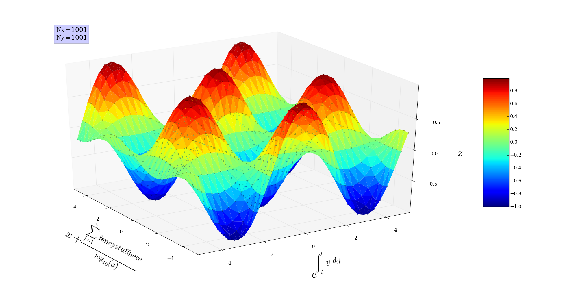
Consider the very simple case that [X,Y] = meshgrid(-5:0.01:5, -5:0.01:5) in Matlab and that we generate the variable Z = sin(X).*cos(Y). Then Nx = Ny = 1001. We then run the following:
X = reshape(X', Nx*Ny, 1);
Y = reshape(Y', Nx*Ny, 1);
Z = reshape(Z', Nx*Ny, 1);
filename = 'stuff.txt';
dlmwrite(filename, [Nx, Ny]);
dlmwrite(filename, [X,Y,Z], '-append');
If we tried to plot every point saved to file in Python or Matlab, we would be in for some serious slowdown. So we can set xskip = 30, yskip = 30 (try experimenting with how small you can make this without leading to an overflow) to reduce the number of points used in a uniform manner. If we run the above python code by typing python plotfigures.py 1, we get the following image after saving as a .png file: